Process sensor and live data with PlexMap
Sensor data or other live data can be displayed as layers in the PlexMap Viewer. The displayed data is automatically updated at the intervals specified in the data source.
One example application is the city-wide bicycle counting stations in Hamburg (see also figure), which display bicycle traffic every 15 minutes.
A prerequisite for successful data integration is that the live data is provided via the OGC standard "SensorThings API."
To successfully integrate live data, you need access to the PlexMap backend and PlexMap 2D or PlexMap 3D.

Import live data to PlexMap Anchor
For processing live data, all Switchboard functions in the livedataset namespace are available. Since not every data import is the same and depends on the specific data provision method, the import described below should be understood as an example.
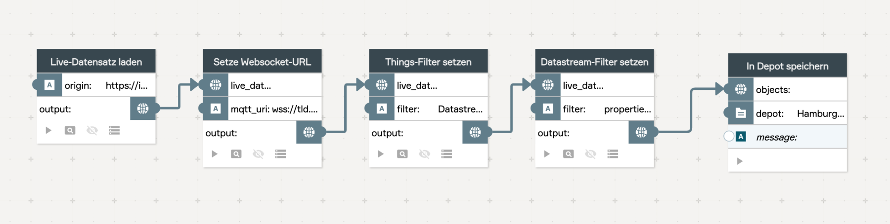
First, the live dataset is loaded using the Load Live Data function. To do this, please specify the URL where the dataset is available under "origin." Load Live Data loads a data source according to the OGC SensorThings v1.1 API as a live dataset.
The websocket URL is now set using the Set websocket endpoint function. This function sets the MQTT over the websocket endpoint for the SensorThings query. The URL entered here must be a websocket URI (ws:// or wss://).
Now use Set Things-Filter to set the filter for the SensorThings Things query, and then use Set Datastream-Filter to set the filter for the SensorThings Datastream query. This can improve the performance of your view.
Finally, use Store in Depot to save the live dataset to a PlexMap depot.
Visualize live data with PlexMap Anchor
The live data you have imported can now easily be stored in a layer using the function Store in Layer.
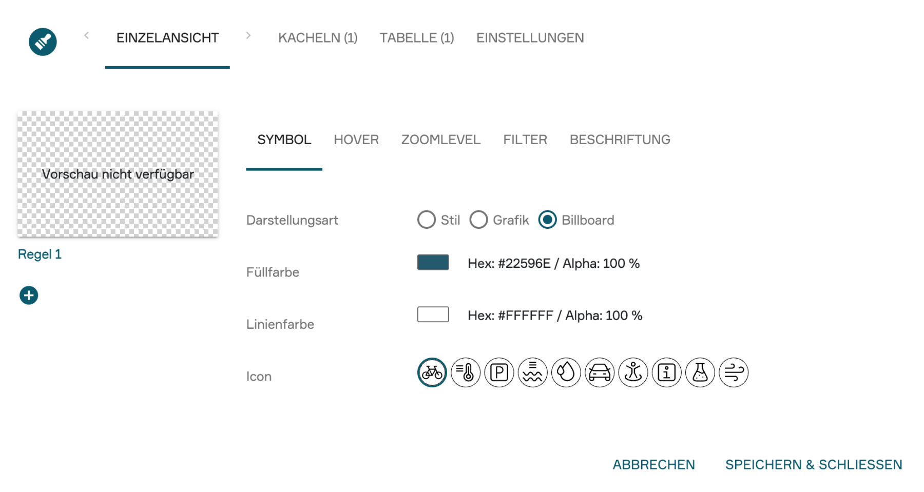
By clicking to the right of the word “style” in the Switchboard function Store in Layer, you can configure the style for displaying your live data (see figure).
In the “Symbol” tab, set the display type to “Billboard” (see figure). You can now choose any fill and line color for the live data query window. If you do not select an icon under “Icon,” only a label will be displayed. If you select an icon here, it will appear centered above your label in the query window.
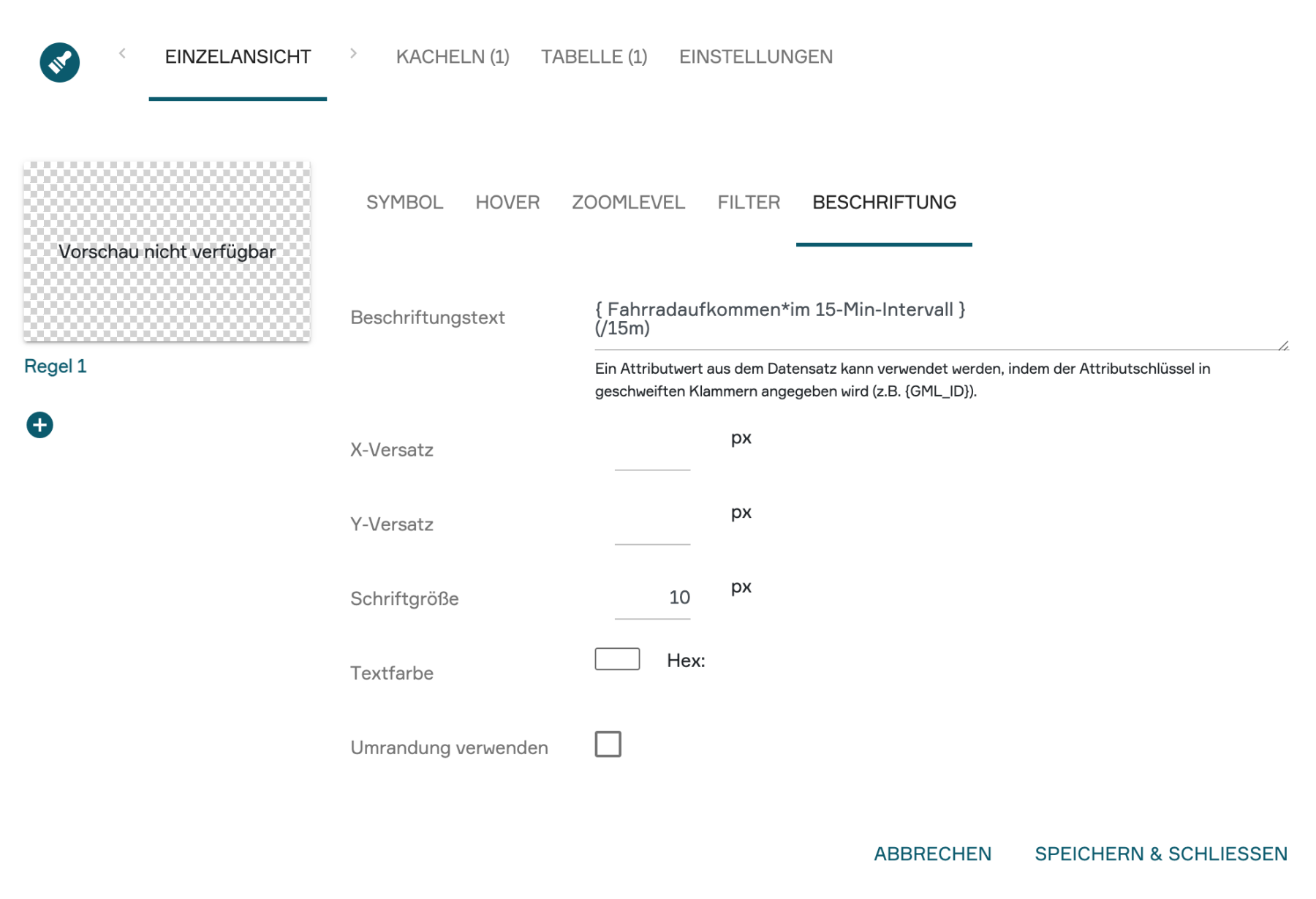
Next, navigate to the “Label” tab (see figure). Under “Label Text,” enter an attribute value from your dataset that should be used for labeling. To do this, specify the attribute key in curly brackets (e.g., {BicycleTraffic*in 15-Min-Intervals}). Also, enter the label for the attribute key that should be displayed in the query window under “Label Text” (here, “(/15m)”). If you want the label to appear directly after the attribute value, do not include a line break. In our example, the label will appear with a line break after the attribute value.
In the additional settings under “Label,” you can adjust the offset, font size, and text color. You can also specify whether to use a border. It is best to start with the default settings and optimize from there.