Toolbox
A comprehensive toolbox is available for use in the PlexMap Viewer. All tools are described in detail below.
Please note that not all tools are available in all map applications and in all view modes.
Coordinates Anchor
The Coordinates tool is all about the geocoordinates of a map. Here you can read coordinates, search for them and much more.

Under "Map center", the coordinate tool displays the geocoordinate of the currently selected map center point.
Furthermore, the displayed coordinates can be converted into various other coordinate systems using the drop-down menu under "Current coordinate system". Which coordinate systems are offered here depends on the individual design of the map you are using.
Furthermore, it is possible to search for coordinates. To do this, enter geocoordinates in the coordinate system selected via "Current coordinate system" and then click on the "Jump to coordinates..." button. The viewer will now align the map center to the entered coordinates.

Measure Anchor
PlexMap provides several measurement tools for. The measurement tools offered are different for each view mode.

Measure point coordinates Anchor
You can use the “Measure point” tool to record and then export measuring points.
Once you have selected “Measure point”, a measurement cross appears on the map. If you now press the left mouse button, a measurement point is captured and listed under “Measure point”. In 3D mode, the position coordinates, the height of the point above mean sea level (MSL) and the relative height above the DTM are measured. Individual designations can be given to the individual measured values using the editing function.
In 2D mode, only the position coordinates are output. As 360° panoramic images are visualised in extended 3D mode, you get the same measurement results as in 3D.
In the last measurement line, you can read off the position and height of the measurement point in real time as you move your mouse over the screen.
All measured coordinates can be downloaded as GeoJSON and used for further processing in an external geoinformation system.
Note: The accuracy of the measured values depends on the accuracy of the geodata used.

Measure line lenght Anchor
Select “Measure line” and then left-click with the mouse. You have now defined the starting point of the measuring line. Further left mouse clicks can be used to record any number of additional interpolation points on the measurement line. Double-click to end the measurement.
Under “Line measurements”, the measured values “Length”, “Horizontal distance” and “Inclination” are listed for each total distance. Length” does not take the terrain surface into account. Horizontal distance” measures the actual distance traveled over the terrain. “Inclination” indicates the inclination between the first and last measuring point. ‘Height’ indicates the difference in height between the first and last point measured on the line. The editing function can be used to give the individual measured values individual names.
In 2D mode and Oblique mode, only the total horizontal length of the line is output. The measurement functions for 360° ponoramic images correspond to those of the 3D mode.
The measured distance can be downloaded as GeoJSON and used for further processing in an external geoinformation system.
Note: The accuracy of the measured values depends on the accuracy of the geodata used.

Measure polygon area Anchor
Select the “Measure area” tool and then left-click with the mouse. You have now defined the starting point of a polygon. Further left mouse clicks can be used to capture any number of additional polygon vertices. Double-click to end the measurement.
Once a polygon has been recorded, the tool outputs the “Area” and “Slope” measurements. The individual surfaces can be given individual names using the editing function.
In 2D mode and Oblique mode, only the total area is output in the horizontal plane. As 360° panoramic images are visualised in extended 3D mode, you get the same measurement results as in 3D.
The measured polygon can be downloaded as GeoJSON and used for further processing in an external geoinformation system.
Note: The accuracy of the measured values depends on the accuracy of the geodata used.

Measure height Anchor
You can use the "Measure height" tool to capture three-dimensional measurement points and then export them.
The “Measure height” tool can be used to record height values along a vertical measurement section and then export them.
Once you have selected “Measure height”, a measuring cross appears on the map. If you now press the left mouse button, the starting point of your vertical measurement section is recorded. Now select a higher point in the 3D viewer and press the left mouse button again. You have now finished capturing the vertical measurement section.
The tool displays the measured vertical distance as “Height” under “Height measurement”.
The tool is available in 3D mode as well as for 360° panoramic images and Oblique mode.
The measured distance can be downloaded as GeoJSON and used for further processing in an external geoinformation system.
Note: The accuracy of the measured values depends on the accuracy of the geodata used.

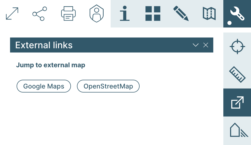
External links Anchor
External map applications (e.g. OpenStreetMap) can be accessed from within PlexMap using the "external links" tool.

By clicking on the offered buttons, the selected external map application is called up at the current geocoordinate/the currently selected map section.
Note: The selection of the offered external map applications is not identical in every map.
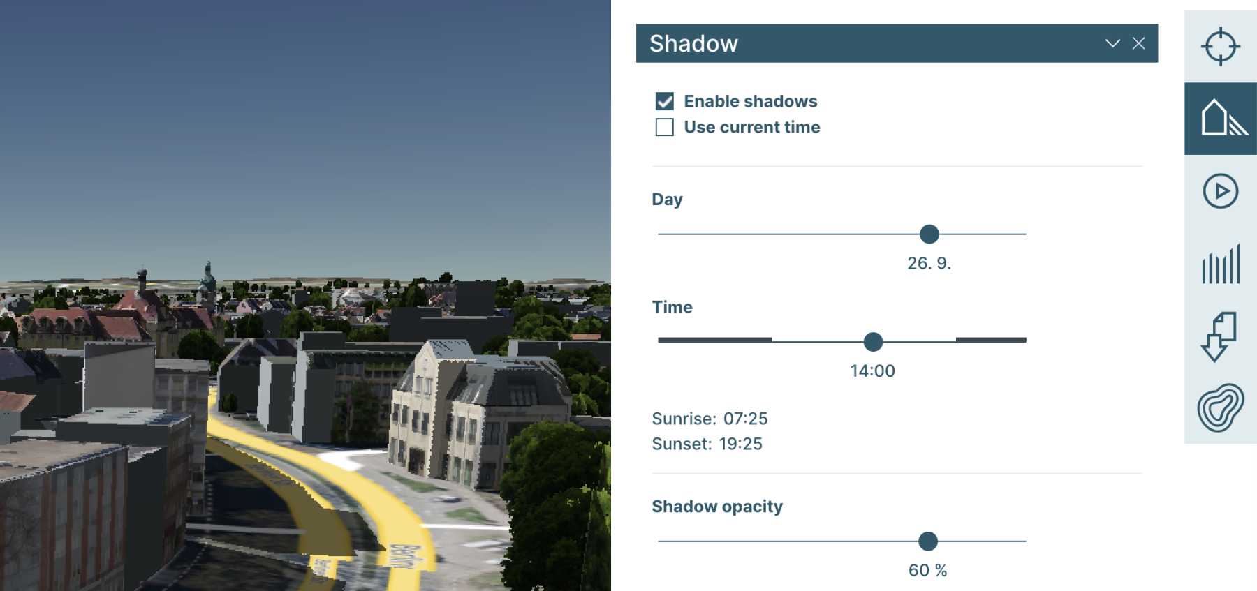
Shading Anchor
Using the "Shading" tool, shading effects can be simulated for any date and time.

To simulate shading, first check "Show shading" at the very top of the tool.
If you check the "Use current time" box, the 3D viewer will display the shading at the current time.
Alternatively, you can use the sliders at "Day" and "Time" to enter a desired date and time. The 3D-Viewer will now display the shading for this time.
The tool will also display the sunrise and sunset times for each selected day.
The brightness of the shadow display can be adjusted using the "Intensity" slider.
Note: The accuracy of the calculated values depends on the accuracy of the geodata used.
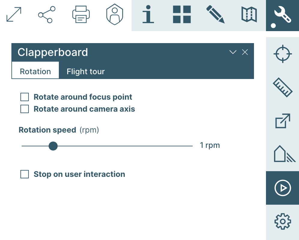
Clapperboard Anchor
Simple rotations and flight tours can be created in 3D mode via the "Clapperboard" tool.

Functions in the "Rotation" tab
Check "Rotate around own axis" to rotate around your own axis in the 3D viewer.
Check "Rotate around focus point" to rotate around the current focus point in the 3D viewer.
You can use the slider under "Rotation speed" to specify the speed of the rotation in revolutions per minute (RPM).
If you place a check mark next to "Stop on user interaction", the 3D viewer will stop the rotation as soon as you move the displayed map section.
Alternatively, you can move the displayed map section at any time and the set rotation will continue.
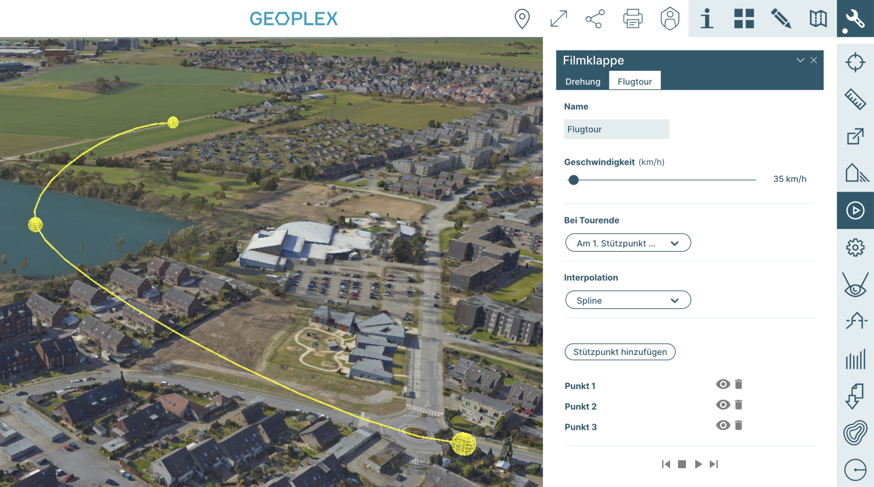
Functions in the "Flight tour" tab
Switch to the tab to access the functions described below.
Under "Flight Tour", a flight tour can be created and played through the 3D viewer. You can use external screen capture software to save a played tour as a video.
First give your tour an appropriate name under "Name". Under "Speed" you can enter a speed in kilometers per hour (km/h) at which the tour will later be flown.
Under "At tour end" you define what should happen at the end of a tour (at the last base). The following options are offered:
Start at first base: If you select this option, the tour will be restarted at the first base point.
Stop: If you select this option, the tour will be stopped and not flown again.
Start tour backwards: If you select this option, the tour will be flown backwards. The camera view is rotated and the points are flown in reverse order.
Fly circuit: If you select this option, the tour will be flown as a circuit. The camera view flies directly from the last to the first base point.
Under "Interpolation" you can define how the viewer calculates the flight distance between the defined support points. The following options are offered:
Spline: The viewer will calculate a curve between the support points to avoid a sharp turn to the next point.
Linear: The viewer will fly over the points strictly one after the other without calculating curves.
To define a tour, click on "Add base point". The Viewer will now define the currently displayed map center point as the base point for your flight tour. Now select other map sections and press "Add base point" again in each case to adopt these map centers as base points for your flight tour.
The defined support points are displayed as a sphere in the 3D viewer. The distance between the support points is displayed as a line.
After you have defined support points, they appear in a list. You can approach individual support points via the displayed eye. You can use the garbage can to delete individual points.
In addition, the following buttons are now displayed for a flight tour:
Back: Jumps to the previous base.
Stop: Stops the flight tour.
Play: Plays the flight tour.
Forward: Jumps to the next base point.
You can make changes to the settings described so far at any time to test them. If you agree with the tour, press "Save tour".
The tour is now displayed under "Interesting Places" on the left side of your map and can be executed there. Changes to the created flight tour are now no longer possible.
If you are logged into PlexMap and have access to the PlexMap backend, you can find the created tour under "Layers" and permanently add it to a map as a Point of Interest (POI).
If you are not logged in as a user in PlexMap or do not have access to the PlexMap backend, the created flight tour will disappear as soon as you reload the viewer.
Render settings Anchor
In the "Render Settings" tool (Display Settings) you can access various options that allow you to influence the map display in PlexMap's 3D mode.
The "Render Settings" are divided into four tabs, which are described below.
Please note that all settings in the "Render Settings" section are valid for one session only. When you reopen the map, all settings will be reset to their respective default values.

Preferences" tab
In the "Preferences" tab you will find various simple display options that we have prepared for you.
Using the slider under "Quality" you can adjust the display quality of the 3D representation. By default, a 3D map is loaded in the "Medium" quality level to ensure an optimal balance between loading performance and the look of your 3D map. Select "Minimal" to reduce detail to optimize loading performance. Select "Maximum" to load all details. Depending on the quality of your internet connection and graphics card, this setting may negatively affect loading performance.
Note: Your setting made in "Quality" is only valid for one session and will not be saved when you reload the map.
Under "Preferences" you will find various display options for the 3D map. Click the radio button to select a preset. It is not possible to combine different presets.
Default: Resets all changes to the default setting you started with in the map application.
Rainy: Simulates rain.
Snowy: Simulates snow.
"Golden Hour": Simulates the "golden hour" just after sunrise or just before sunset.
"Blue Hour": Simulates the "blue hour". The term blue hour refers to the period of time within the evening or morning twilight during which the sun is so far below the horizon that the blue light spectrum in the sky is still or already dominant and the darkness of the night has not yet arrived or has already passed.
Black and white: Colors the map display black and white.
Drawing Style: Converts the map display into a comic-like drawing style.
Close-up: Creates a close-up for the current map section.
Wide Angle: Creates a wide angle image for the current map section.

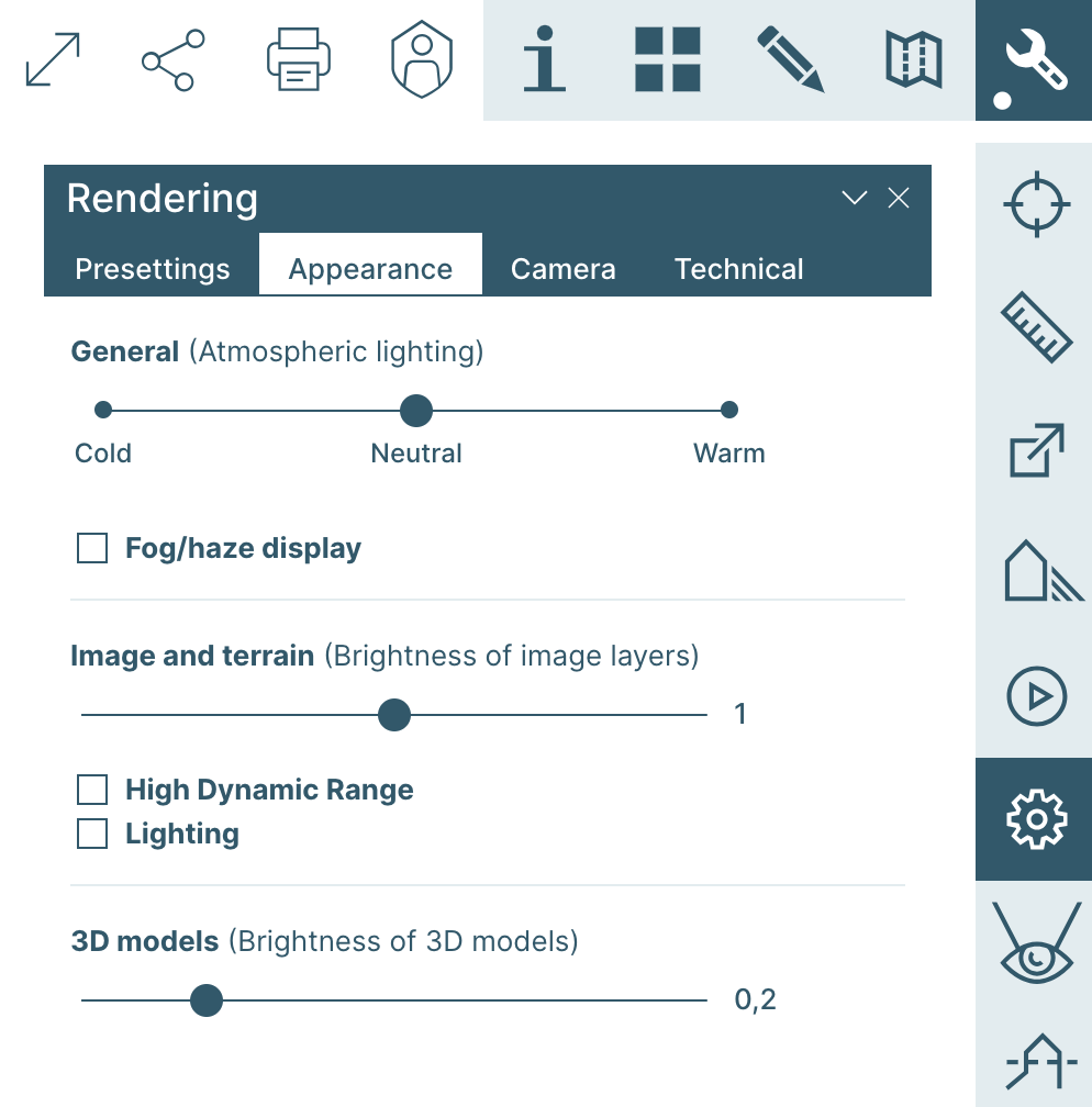
"Appearance" tab
Various display options can be configured in the "Appearance" tab.
The slider under "General (Atmospheric Lighting)" can be used to set the lighting of the 3D display to "cold", "neutral" or "warm". "Neutral" is the standard illumination with which you have called up the 3D viewer. "cold" increases the blue and "warm" the yellow values in the map display.
If you check "fog/haze", objects further away will disappear in a fog.
The slider under "Image and Terrain (Brightness of Image Layers)" can be used to adjust the brightness of image layers (e.g. aerial images). The default value is "1". The maximum brightness can be reached by setting the slider to "2". The minimum brightness is reached at the value "0".
If you check "High Dynamic Range", an HDR display will be calculated for the image layers (e.g. aerial images). A check mark at "Illumination" puts a shadow on the image layers.
The slider under "3D models (brightness of 3D models)" can be used to influence the brightness of the displayed 3D models. The default value here is "0.2". If you set the brightness of the 3D models to "0", 3D models will be displayed very darkly. If you set the value to "1", the displayed 3D models will be very brightly illuminated.
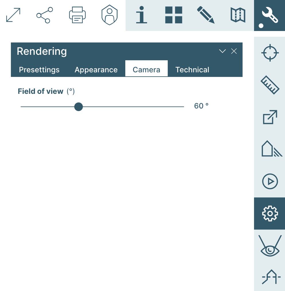
"Camera" tab
In the "Camera" tab, the "Field of view (°)" slider can be used to specify the displayed field of view in degrees. By default, the field of view is limited to 60 degrees. If you set the value to the minimum value of 5 degrees, the displayed field of view will be restricted accordingly. Using the maximum value of 160 degrees, the field of view can be extended to 160 degrees.
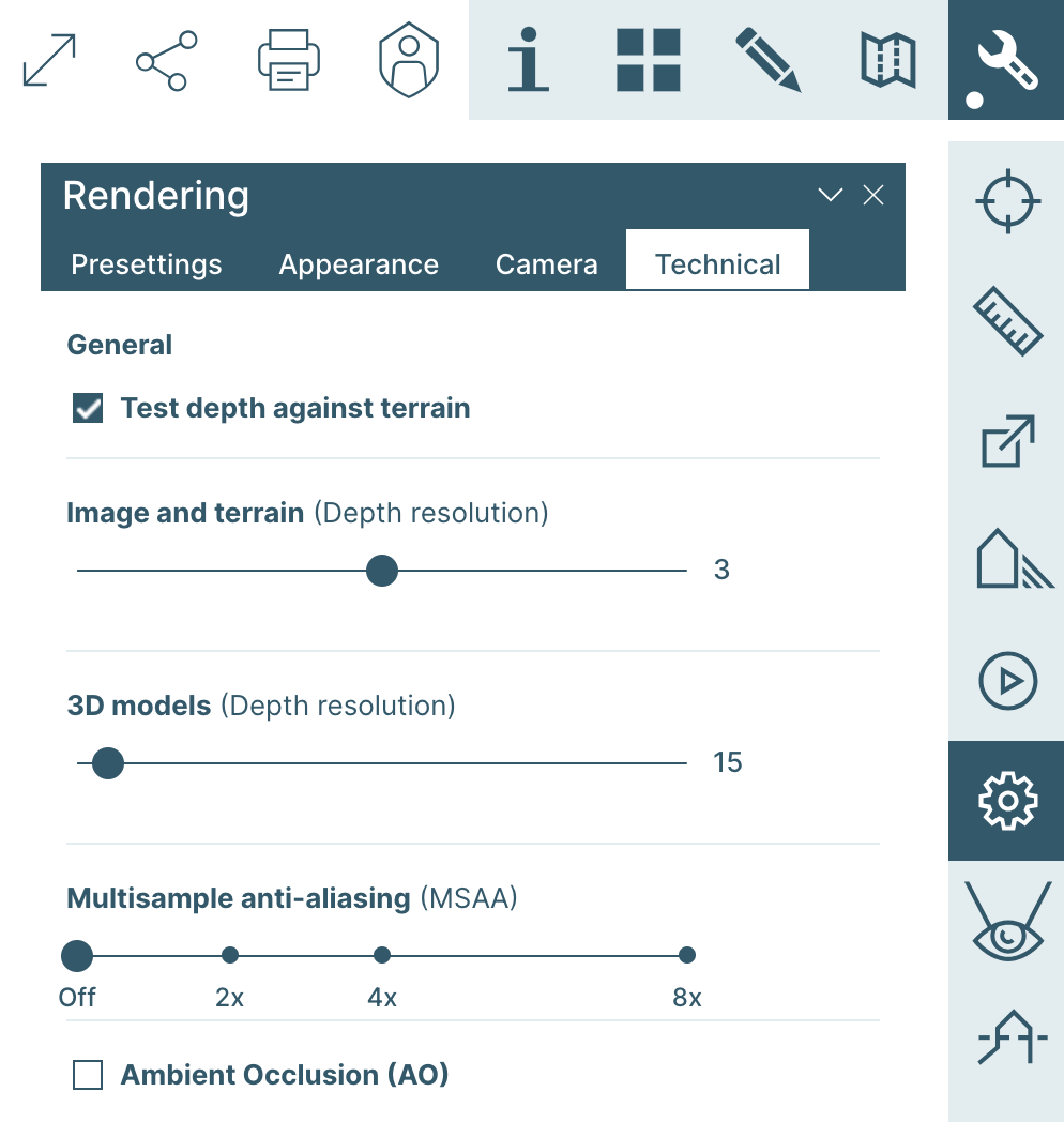
"Technical" tab
Various technical settings can be made in the "Technical" tab. You should ignore these settings if you are not an expert user.
If "Test depth against terrain" is checked, the terrain (the 3D terrain) will shine through a displayed 3D surface (e.g. a 3D mesh) in some places. If the check mark is not set, this is not the case. Please note that for tools like "Measure" or the PlexMap Planner "Test depth against terrain" must be set.
Using the slider under "Image and Terrain (Depth Resolution)" you can set the depth resolution of the displayed image and terrain layers. With a low value (minimum value = 1), less details are loaded for all image and terrain layers. With a higher value (maximum value = 5), the viewer loads more details of the image and terrain layers.
You can use the slider under "3D models (depth resolution)" to set the depth resolution of the displayed 3D models. With a low value (minimum value = 5), less details of the displayed 3D models are loaded. With a higher value (maximum value = 200), the viewer loads more details of the displayed 3D models.
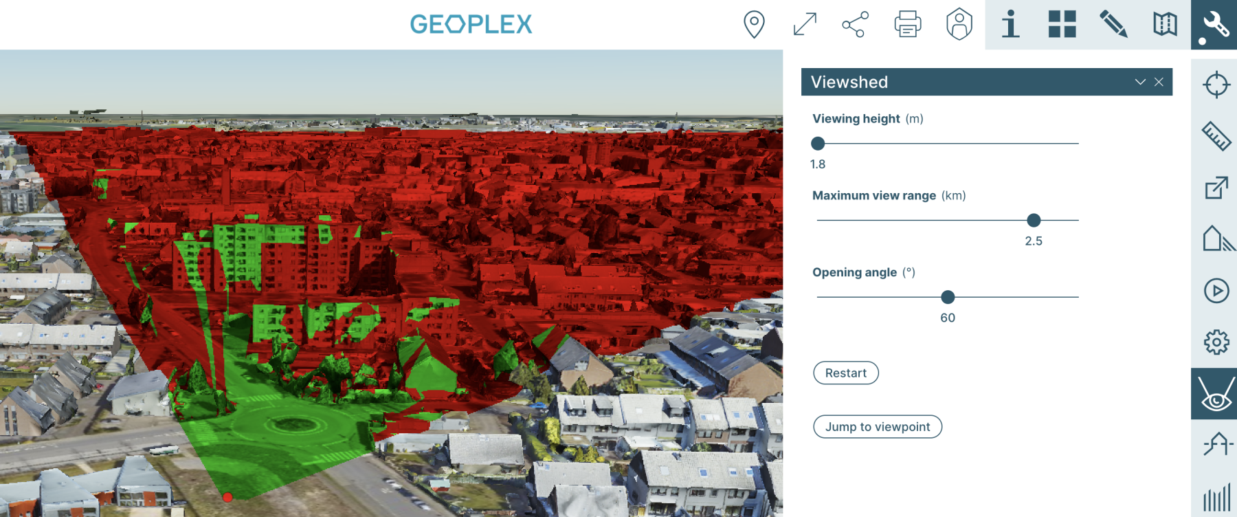
Viewshed Anchor
In the Viewshed tool, visibility relationships can be analyzed and displayed. A viewshed is the geographic area that is visible from a location.

Using the slider under "Viewing height (m)", you can enter the height from which the visibility analysis is to be performed. The tool is preset to 1.8 meters (visibility height of a human). The minimum value is 1 meter the maximum value is 300 meters.
Using the slider under "Maximum visibility (km)", you can set the distance to which the visibility analysis should be performed. The default setting is 2.5 kilometers. The minimum value is 0.1 kilometers and the maximum value is 3 kilometers.
Using the slider under "Opening angle (°)", you can set how large the opening angle should be in degrees. The default setting is 60 degrees. The minimum value is 20 degrees the maximum value is 100 degrees.
To perform a visibility analysis, click on the "Start" button. A red sphere will now appear over your mouse pointer in the 3D viewer. Now find the location from which you want to start the visibility analysis and then press the left mouse button. The field of view and a green sphere with which you can set the viewing direction will now appear. With another left mouse click you can set the viewing direction. Green colored areas are visible from the selected point, red colored points are not visible. The visibility analysis is now complete.
Use the "Restart" button to start a new visibility analysis. You can jump to the selected visibility position using the "Jump to visibility position..." button. From this position, all areas are colored green and are therefore visible.
Cut surface Anchor
You can use the slice tool to place and move layers through the 3D viewer.

After you have selected the slice tool, a blue plane appears in the 3D viewer.
By moving the slider under "Layer height (meters above normal zero)" you can change the height of the layer. Moving the slider under "Opacity (%)" causes a higher or lower opacity of the layer.

Elevation profiles Anchor
The elevation profile tool allows you to create elevation profiles of the terrain or surface in the 3D viewer.

In the tool, first select the basis on which you want to create a height profile.
If you select "Surface profile", the terrain and all objects displayed on it (e.g. trees or buildings) are taken into account in the height profile. If you select "Terrain Profile", only the terrain will be considered in the elevation profile.
After selecting the elevation profile tool, a blue sphere appears in the 3D viewer. Press the left mouse button to set the first piece point of your elevation profile. By further left mouse clicks you can add as many support points as you like. Make a double click to finish the acquisition of your height profile.
The tool now outputs the following measured values for your route:
As the crow flies: gives the measured as the crow flies. Differences in altitude are not taken into account.
Inclined distance: Indicates the measured inclined distance. In contrast to the air line, the height difference between the first and the last support point is taken into account here.
Altitude (minimum): Specifies the lowest elevation along the drawn line.
Altitude (Maximum): Specifies the maximum height along the drawn line.
Height difference: Specifies the difference between the measured minimum and maximum heights.
Elevation: Below the measured values the generated elevation profile is displayed in a line diagram. If the measured height differences are very small, PlexMap will superelevate the display in the diagram. By entering a number in the field to the right of "Superelevation" you can set the factor of superelevation. If the value is "1", the plot will not be superelevated.
If you click on the printer icon, a PDF is exported that contains all measured values and various map representations. You can now print the document or save it as a PDF file.

Export Anchor
The Export tool allows you to export map objects in various data formats.

After you have selected the export tool, please click on the icon with the dashed area.
Now a blue sphere appears over your mouse pointer. You can now draw an area (polygon) within which the displayed geodata are to be exported. To capture the first base point of the polygon, make a left mouse click. By further left mouse clicks you can add as many further supporting points as you like. By a double click you finish the acquisition of the polygon.
The tool will now output the selection area in square meters and the number of selected objects (pieces). The tool will export all objects that at least touch the defined polygon.
Using the drop-down menu under "Export format", you now select the desired data format for your export. The export tool basically supports all formats listed here. Depending on the configuration of a map application, not all listed formats may be available in the tool.
Then click on the "Export selection" button. The exported objects will be saved in the download folder of your end device.
Please note that usually not all layers of a map are also exportable. The tool will export all currently active map layers, provided that the publisher of your map allows an export of the selected map layer.

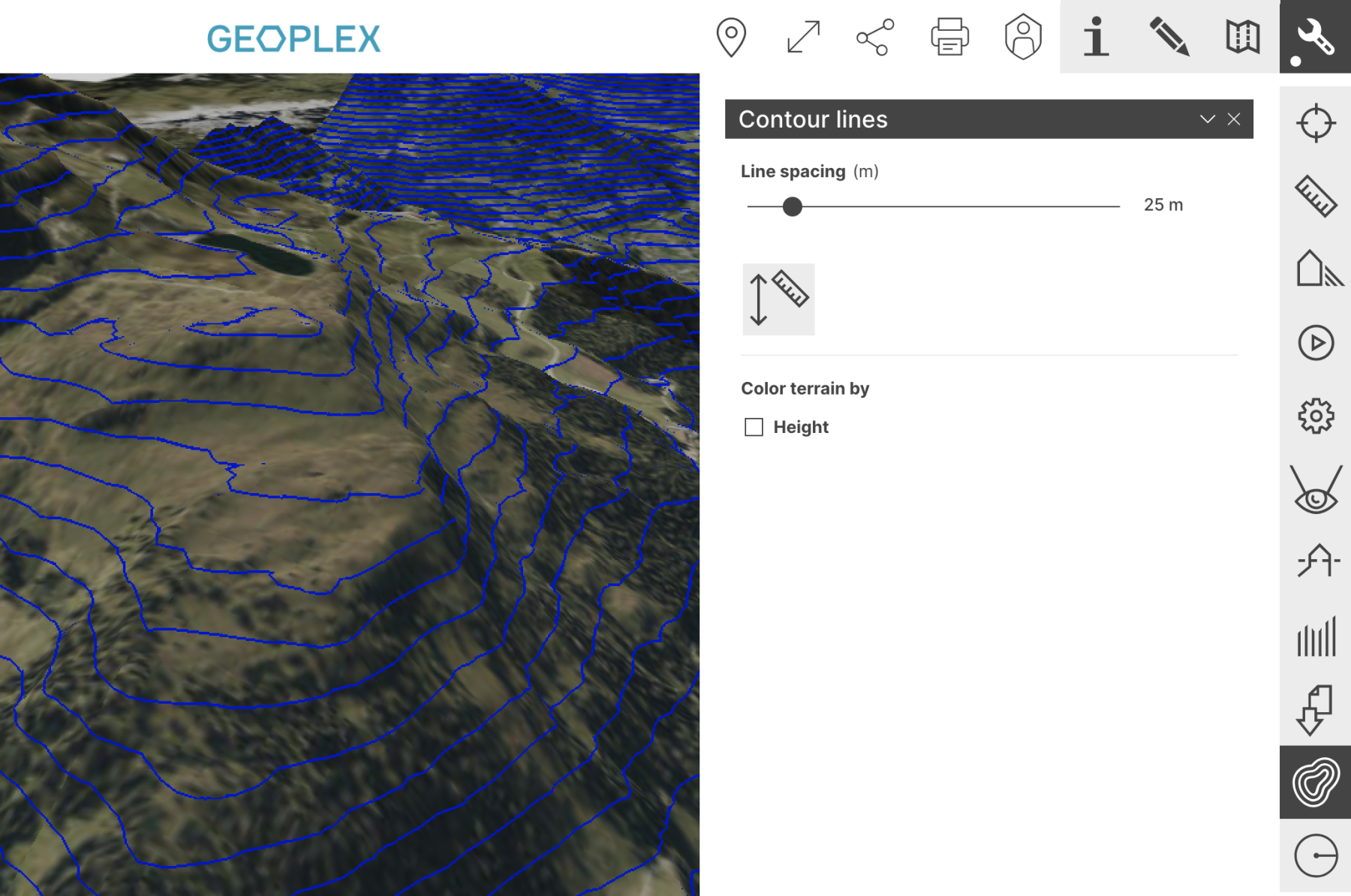
Conturlines Anchor
With the contour line tool you can create contour lines in the 3D viewer and colour the terrain according to height.

After you have opened the tool, you can define the distance between the individual contour lines via the slider under "Line spacing (m)". The contour lines are now displayed in the 3D viewer as blue lines at the desired distance.
By clicking on the button "Query height" you can query the height of the displayed terrain at any point in the 3D-Viewer. To do this, simply move the mouse over the terrain surface after you have selected the "Query height" button. The measured values are queried live and displayed in the viewer. Press the button "Query height" again to end the measurement.
If you tick the "Altitude" box, you can colour the terrain according to altitude. Mountains are now coloured red, valleys blue.
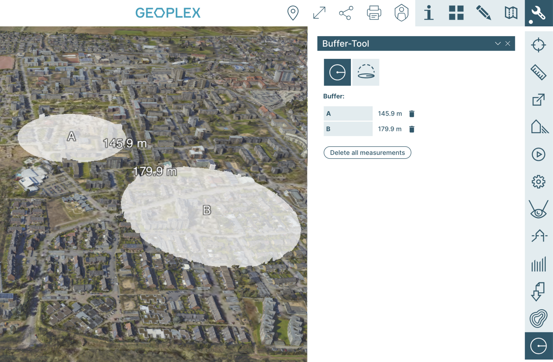
Buffer Anchor
With the buffer tool you can create two- and three-dimensional buffers in the 3D viewer.

After opening the tool, select the button "Draw 2D buffer" or "Draw 3D buffer" to draw a two- or three-dimensional buffer.
Now perform a left mouse click in the map to define the centre point of your buffer. If you now move the mouse away from the set centre point of the buffer, a buffer is shown in the viewer. Finish drawing the buffer with another left mouse click.
If you now press the left mouse button again in the map, you can draw as many more buffers as you like.
Below the buttons "Draw 2D buffer" and "Draw 3D buffer" all drawn buffers are listed. The radius of each buffer is shown in metres. You can delete a buffer by clicking on the bin icon. By clicking on the button "Delete all measurements", you can delete all buffers at the same time.